pacman::p_load(DT,
               readxl,
               CGPfunctions,
               ggHoriPlot,
               lubridate,
               ggthemes,
tidyverse)Take-home Ex04
1 Overview
For this assignment, the impact of COVID-19 as well as the global economic and political dynamic from 2020 to 2022 on Singapore bi-lateral trade will be uncovered with visual analytics. Dataset is taken from Department of Statistics Singapore.
2 Libraries Loading
For this exercise,
readxl is the package for data importing from excel files
CPGfunctions is the package for slopegraph plotting
ggHoriPlot is the package for horizontal graph plotting
tidyverse is the main package for data processing
Other packages are for make-up or minor usage mainly
3 Data Loading
Trade data downloaded from the website is in Excel spreadsheet format.
trade_export_temp <- read_excel("Data/Merchandise trade by region_market.xlsx",
                       sheet = "T1")

trade_import_temp <- read_excel("Data/Merchandise trade by region_market.xlsx",
                       sheet = "T2")
Taking the first look at the data, the table is messy with rows that are not needed. The import and export data tables are separated into two tables at the moment.
DT::datatable(trade_import_temp,
              class = "cell-border stripe")
4 Data Processing
We will therefore remove those irrelevant rows and promote the “Data Series” row as our table title.
To consolidate the export and import tables, a column with the column name “trade” will be tagged to each row, whereby whether the row belongs to “Export” or “Import” will be categorised.
colnames(trade_import_temp) <- as.character(unlist(trade_import_temp[9,]))
colnames(trade_export_temp) <- as.character(unlist(trade_export_temp[9,]))


trade_export_temp <- trade_export_temp[c(11:(nrow(trade_export_temp)-23)),]
export_vector <- rep("Export",
                     nrow(trade_export_temp))

trade_export_temp$trade <- export_vector

trade_import_temp <- trade_import_temp[c(11:(nrow(trade_import_temp)-23)),]
import_vector <- rep("Import",
                     nrow(trade_import_temp))

trade_import_temp$trade <- import_vector


names(trade_export_temp)[1] <- "Market_"
names(trade_import_temp)[1] <- "Market_"
For this exercise, the period of January 2020 to December 2022 is to be studied.
Therefore, only columns of months from 2020, 2021 and 2022 are identified and kept.
trade_export_unpiv <- trade_export_temp[,c(1, 3:38, ncol(trade_export_temp))]
trade_import_unpiv <- trade_import_temp[,c(1, 3:38, ncol(trade_import_temp))]
With that, tables of export and import data are merged together. Columns of trade data by months are gathered (pivoted) into one column. Noticed that some of data are in the unit of millions while some are in thousands. To ensure data consistency, we will make adjustments by translating all data into the unit of dollar.
trade_full <- rbind(trade_export_unpiv,
                    trade_import_unpiv) %>%
  gather(key = "Month_", value = "Trade_Amount", -Market_, -trade) %>%
  mutate(month_num = ym(Month_))


trade_full$`Trade_Amount` <- as.numeric(trade_full$`Trade_Amount`)

trade_full$`Trade_Amount` <- ifelse(grepl("Thousand Dollars", trade_full$Market_), trade_full$'Trade_Amount' * 1000, trade_full$'Trade_Amount' * 1000000)

trade_full$Market_ <- gsub(" \\(Thousand Dollars\\)|\\(Million Dollars\\)", "", trade_full$Market_)
The column of “Month_” is split into “Year” and “Month” for convenience.
trade_clean <-
separate(trade_full,
         Month_,
         into = c("Year", "Month"),
         sep = " ",
         convert = TRUE,
         remove = TRUE)

trade_clean$Trade_Amount <- ifelse(is.na(trade_clean$Trade_Amount), 0, trade_clean$Trade_Amount)


month_order <- c("Jan", "Feb", "Mar", "Apr", "May", "Jun",
                 "Jul", "Aug", "Sep", "Oct", "Nov", "Dec")

trade_clean$Month <- factor(trade_clean$Month, levels = month_order)

DT::datatable(trade_clean,
              class = "cell-border stripe")
A table of trade_clean but in wide format is also produced and saved inside the “diff” column for net export trade calculation.
trade_clean_wide <- trade_clean %>%
  pivot_wider(names_from = trade,
              values_from = Trade_Amount)


trade_clean_wide$diff = trade_clean_wide$Export - trade_clean_wide$Import
5 Visual Analysis
5.1 Trade volume from different continents
A slopegraph of total trade volume with Singapore from each of continents is produced below for the period of 2020 to 2022 during the pandemic.
The slopegraph is chosen as it is capable of revealing the trade volumes change between two time points.
trade_region <- trade_clean %>%
  filter(trimws(Market_) %in% c("America", "Asia", "Europe", "Oceania", "Africa"))
p1 <- trade_region %>%
group_by(Market_, Year) %>%
summarise(Trade_Total = round(sum(Trade_Amount) / 1000000000, 2)) %>%
mutate(year = factor(Year)) %>%
newggslopegraph(year, Trade_Total, Market_,
LineThickness = 0.75,
YTextSize = 4,
Title = "Trade Volume by continents (in $Billions)",
SubTitle = "From 2020 to 2022",
Caption = "Total trade value is the sum of export from and import to Singapore") +
labs(y = "Total trade value ($Billions)",
x = "Year") +
theme_economist() +
theme(legend.position = "null",
axis.title.y = element_text(vjust = 2.5),
plot.title = element_text(vjust = 2.5))
p1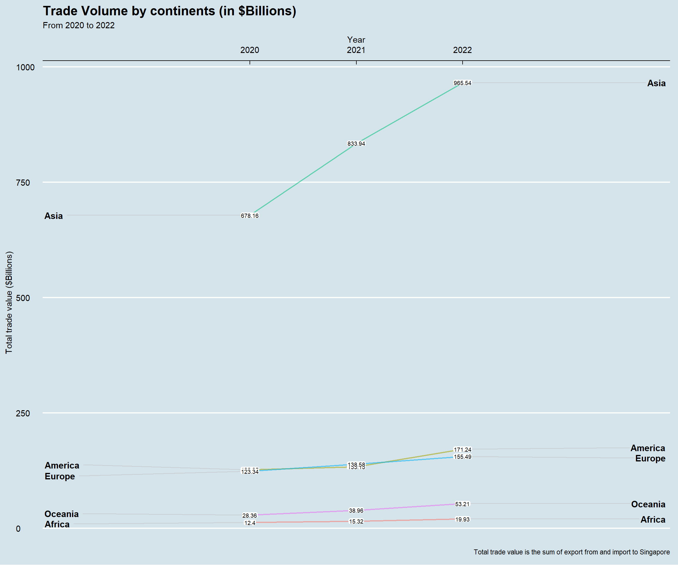
5.2 Singapore’s trade surplus/deficit with the top 10 trade volume countries
A positive balance of trade, known as a trade surplus, occurs when a country exports more goods than it imports. This usually means the country is earning more from its exports than it is spending on its imports, and it is generally seen as a sign of economic strength. On the other hand, trade deficits occurs when a country imports more goods than it exports.
Here, we will look at the top 10 countries of trade volumes with Singapore in 2022 and their trade balance during the 3-year span. A horizontal plot is chosen here to enable readability with sufficient horizontal space.
trade_top10country_2022 <- trade_clean %>%
  filter(!trimws(Market_) %in% c("America", "Asia", "Europe", "Oceania", "Africa", "European Union")) %>%
  filter(Year == 2022) %>%
  group_by(Market_, Year) %>%
  summarise(Trade_Total = round(sum(Trade_Amount) / 1000000000, 2)) %>%
  arrange(desc(Trade_Total))
top10_2022 <- head(trade_top10country_2022$Market_, 10)
p2 <- trade_clean_wide %>%
filter(Market_ %in% top10_2022) %>%
ggplot() +
geom_horizon(aes(x = month_num,
y = diff),
origin = 0,
horizonscale = 8) +
facet_grid(Market_ ~.) +
geom_vline(xintercept = as.numeric(as.Date("2021-1-1")),
color = "black",
linetype = "dashed",
linewidth = 0.5) +
geom_vline(xintercept = as.numeric(as.Date("2022-1-1")),
color = "black",
linetype = "dashed",
linewidth = 0.5) +
theme_economist() +
scale_fill_hcl(palette = 'RdBu') +
theme(panel.spacing.y = unit(0, "lines"),
strip.text.y = element_text(size = 10,
angle = 0,
hjust = 0.5),
legend.position = 'none',
axis.text.y = element_blank(),
axis.text.x = element_text(size = 10,
angle = 0,
hjust = 0.5),
axis.title.y = element_blank(),
axis.title.x = element_blank(),
axis.ticks.y = element_blank(),
panel.border = element_blank()
) +
ggtitle('Net Export from Top 10 Total Trade Value Countries with Singapore') +
labs(subtitle = "Net Export = Export - Import. Blue means Surplus, red means deficit.")
p2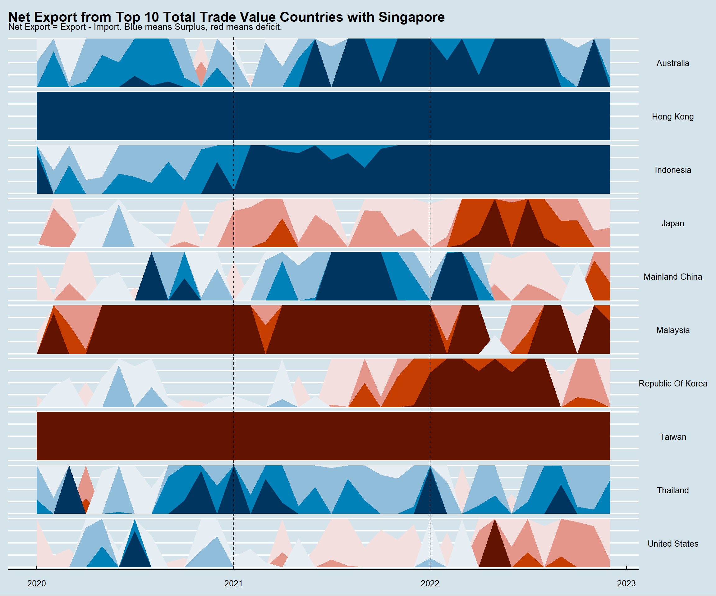
5.3 Top 10 trading countries monthly trade volume (2020 to 2022)
We are also interested in the trend of the trade volume by month from each of the top 10 countries, to see if there is any seasonality pattern. A cycle plot is captured to present how values vary over a period of time.
trade_cycle <- trade_clean %>%
  filter(Market_ %in% top10_2022) %>%
  mutate(Trade_Amount = Trade_Amount / 1000000) %>%
  group_by(Market_, Month, Year) %>%
  summarise(total_trade_amt = sum(Trade_Amount))


p3 <- ggplot(data = trade_cycle) +
  geom_line(aes(x = Year,
                y = total_trade_amt,
                group = Market_,
                color = Market_)) +
  geom_text(data = . %>%
              group_by(Market_) %>%
              filter(Year == max(Year)),
            aes(x = Year,
                y = total_trade_amt,
                label = Market_),
            nudge_x = 0,
            nudge_y = 0,
            hjust = 0.95,
            size = 3.5) +
  scale_x_continuous(breaks = seq(2020, 2022, 1),
                     labels = c("2020", "2021", "2022")) +
  facet_wrap(~Month,
             ncol = 6) +
  theme_economist() +
    labs(title = "Top 10 trading countries trade volume by month (2020 to 2022)",
         y = "Total Trade Amount ($millions)",
         x = NULL) +
    theme(plot.title = element_text(vjust = 2.5),
          legend.position = "none",
          axis.title.y = element_text(vjust = 2.5),
          panel.spacing.x = unit(0.9, "line"))
p3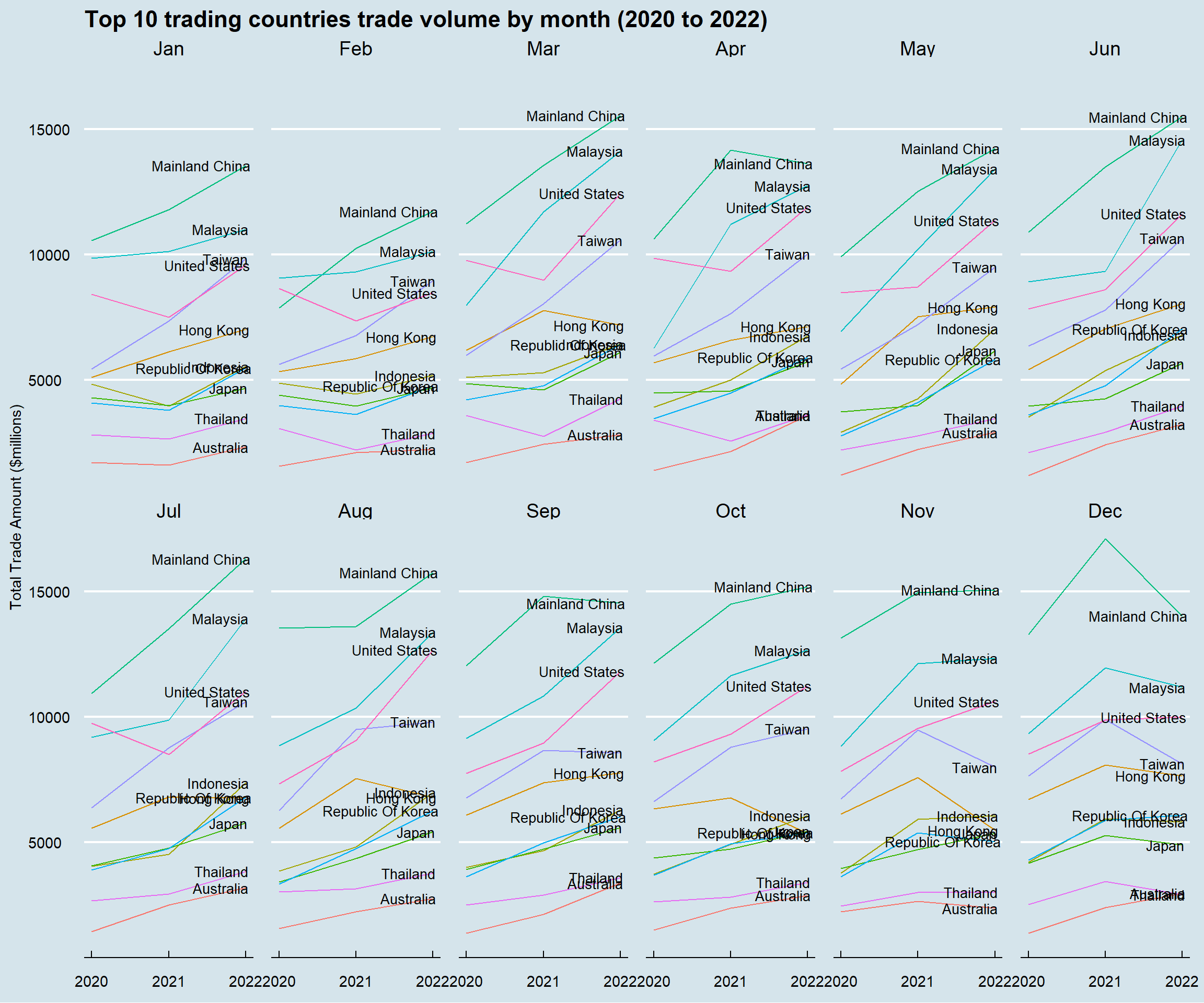
6 Insights and thoughts
i. Singapore’s bi-lateral trade with the rest of the world is in the process of recovering from the impact of COVID-19 and global economic and political dynamic. Across the five continents, an upward trend is observed from 2020 to 2022, as seen in Figure 1
ii. The bulky portion of Singapore’s bi-lateral trade comes from Asia. According to Figure 3,
Mainland China is undoubtedly the biggest contributor.
Malaysia, Taiwan, Hong Kong and Indonesia are the rest of top 5 trade partners from Asia.
iii. Trade deficit is constantly observed from Singapore’s partnership with Japan, Malaysia and Taiwan, while a consistent surplus is observed from the trade partnership with Australia, Hong Kong, Indonesia, using the color from Figure 2
iv. The trade volume is rather consistent throughout the year for different months, with the exception of February, in which a lower value is observed for most Asian selected countries in all three years. This could be largely due to two main reasons:
There are usually less number of days in the calendar month of February.
Most of Chinese New Year holidays fall in the month of February, both sides’ work and operations could be in a slower pace as compared to the rest of months.